testing whether a coin is fair
2022-03-06 · 6 min read
Source: https://www.wikiwand.com/en/Checking_whether_a_coin_is_fair
- good problem for applying principles of statistical inference
- good problem for comparing different methods of statistical inference.
for inference, the key questions
- how many trials should we take?
- given some # of trials, how accurate is our estimate of
Pr[H]?
more rigorously, the problem is about determining the parameters of a Bernoulli process given only a limited # of trials.
this article covers two methods (of many):
-
Posterior PDF (Bayesian approach)
init: true p_H unknown. uncertainty represented by prior distribution. posterior distribution obtained by combining prior and likelihood function (represents information obtained throught the experiment).
p_fair can be obtained by integrating the PDF of the posterior over the "fair" masses?
Bayesian approach is biased by prior (which could be good if it's accurate).
-
Estimator of true probability (Frequentist approach)
assumes experimenter can toss the coin however many times they wish. first, you decide on a desired level of confidence and tolerable margin of error, which give you the minimum number of tosses needed to perform the experiment.
Posterior PDF #
TODO
Estimator of true probability #
This method depends on two paramters:
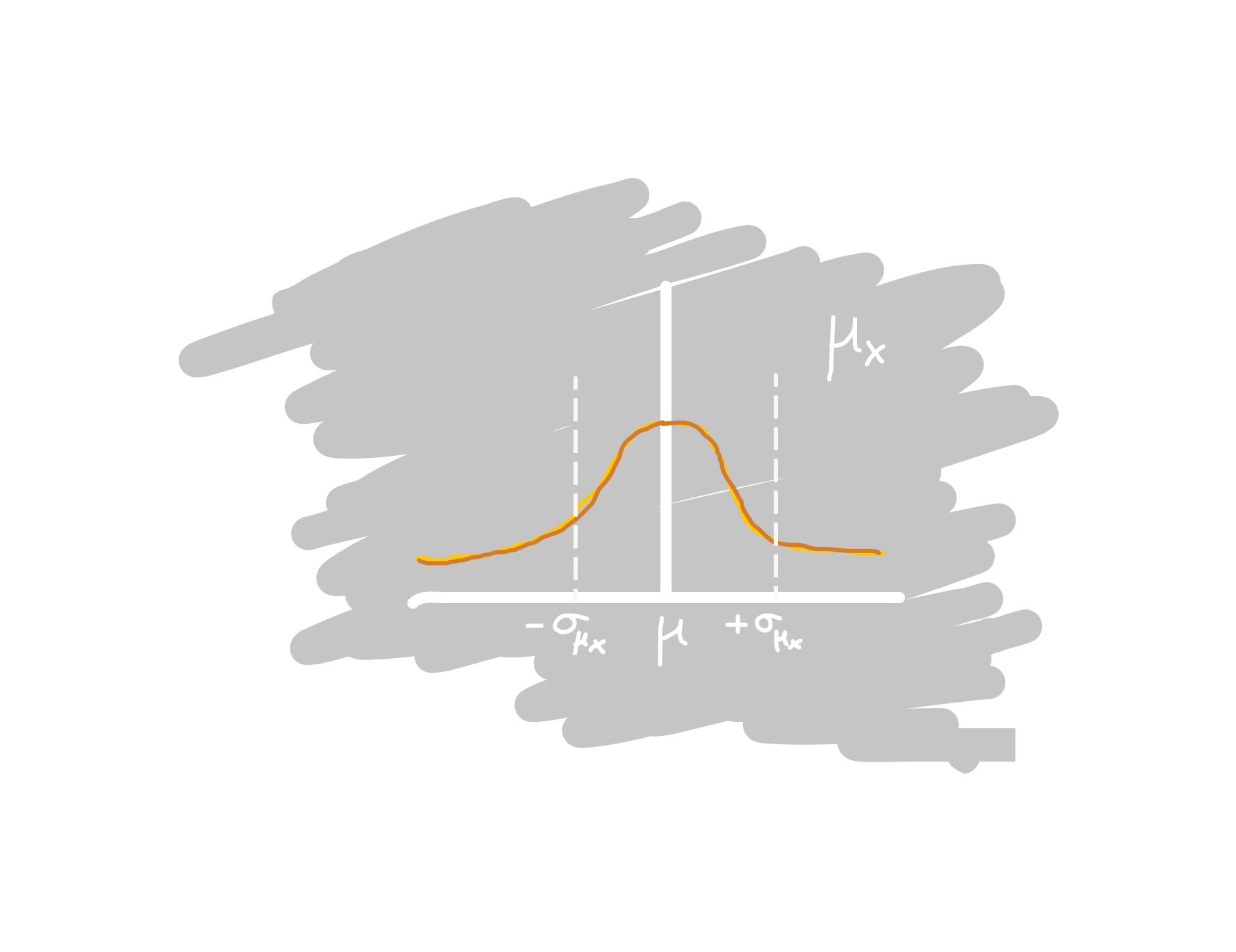
- ($Z$) the confidence level, given by a Z-value of the standard normal distribution. Recall that $Z = \frac{\mu_x - \mu}{\sigma_{\mu_x}}$, i.e., deviation of the sample mean $\mu_x$ from the population mean $\mu$, divided by the standard error of the mean $\sigma_{\mu_x}$. Intuitively, if the sample mean deviates by exactly "one sigma", the Z-value is then 1.0.
- ($E$) the maximum acceptable error
Some example $Z$-values:
| $Z$-value | Confidence level | Comment |
|---|---|---|
| 0.6745 | 50.000% | |
| 1.0000 | 68.269% | $\sigma$ |
| 1.9599 | 95.000% | |
| 3.2905 | 99.900% | "three nines" |
| 4.0000 | 99.993% | $4 \cdot \sigma$ |
| 4.4172 | 99.999% | "five nines" |
Let $r$ be the actual probability of obtaining heads. Let $p$ be the estimated probability of obtaining heads.
Here, we just use the MLE for $p$, i.e., $p = \frac{h}{h + t}$ with naximum margin of error $E > |p - r|$.
Recall, the standard error, $s_p$, for the estimate $p$ is: $$ s_p = \sqrt{\frac{p \cdot (1-p)}{n}} $$
The maximum error is given by $E = Z \cdot s_p$, but we can simplify this with an approximation:
Notice that $s_p$ is greatest when $p = (1 - p) = 0.5$. It follows then that $s_p \le \sqrt{\frac{0.5 \cdot 0.5}{n}} = \frac{1}{2 \sqrt{n}}$. Consequently, $E \le \frac{Z}{2 \sqrt{n}}$.
The maximum required number of trials $n$ then follows:
$$ n \le \frac{Z^2}{4 \cdot E^2} $$
Examples #
| $E$ | $Z$ | $n$ |
|---|---|---|
| 0.1 | 1.0 | 25 |
| 0.1 | 2.0 | 100 |
| 0.1 | 3.0 | 225 |
| 0.1 | 4.0 | 400 |
| 0.1 | 5.0 | 625 |
| 0.01 | 1.0 | 2500 |
| 0.01 | 2.0 | 10000 |
| 0.01 | 3.0 | 22500 |
| 0.01 | 4.0 | 40000 |
| 0.01 | 5.0 | 62500 |
| 0.001 | 1.0 | 2.50e5 |
| 0.001 | 2.0 | 1.00e6 |
| 0.001 | 3.0 | 2.25e6 |
| 0.001 | 4.0 | 4.00e6 |
| 0.001 | 5.0 | 6.25e6 |
General Case #
Consider the distribution of the sample mean, $\mu_x$, (assuming we took many samples with $n$ trials each). Note the population mean $\mu$ and the standard error of the mean, $\sigma_{\mu_x}$ (the stddev of the sample mean).
One interesting question is: given a fixed number of trials, say $n = 1000$, what should our maximum tolerated absolute deviation, $E$, be? What is our key parameter for choosing a good $E$?
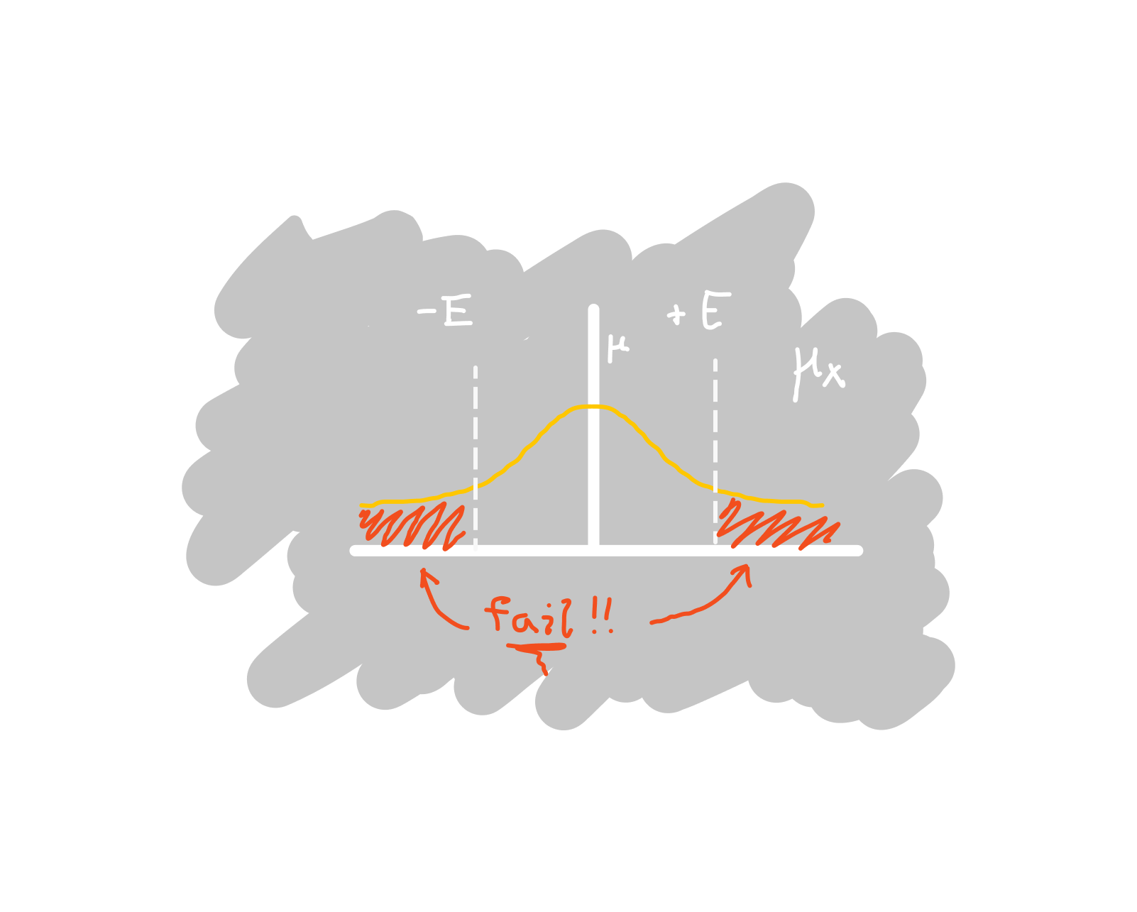
We should choose $E$ based on our required confidence. Given that the samples are actually drawn from the population, we want some small probability of failure (or inversely, a large probability of success), where our statistical criterion decides that the samples are not actually drawn from the population.
Using the maximum absolute deviation $E$ as a criterion, we will claim the two distributions are not the same if the sample mean $\mu_x$ lies within the red "fail" zone above.
More precisely, our failure probability is the probability that $\mu_x$ is outside of the interval $[\mu - E, \mu + E]$:
$$ Pr[failure] = Pr[(\mu_x < \mu - E) \cup (\mu + E < \mu_x)] $$
Since the sample mean is normal (law of large numbers), the upper and lower probabilities are identical, so we can simplify as
$$ Pr[failure] = 2 \cdot Pr[\mu_x < \mu - E] = 2 \cdot F_\mu(\mu - E) $$
where $F_\mu$ is the CDF of the normal distribution $N(\mu, \sigma_{\mu_x})$. By normalizing the interval bounds in terms of the standard normal distribution, we can see
$$ Pr[failure] = 2 \cdot \Phi\left(\frac{(\mu - E) - \mu}{\sigma_{\mu_x}} \right) = 2 \cdot \Phi\left(\frac{-E}{\sigma_{\mu_x}} \right) $$
where $\Phi$ is the CDF of the standard normal distribution. Given a desired $p_f = Pr[failure]$, we can compute the error bounds $E$
$$ \begin{align*} p_f &= 2 \cdot \Phi\left(\frac{-E}{\sigma_{\mu_x}} \right) \ \frac{-E}{\sigma_{\mu_x}} &= \Phi^{-1}(p_f / 2) \ E &= -\sigma_{\mu_x} \cdot \Phi^{-1}(p_f / 2) \ \end{align*} $$
Of course, it can be annoying to compute the inverse normal CDF, so it's often useful to frame $p_f$ in terms of the Z-score, or "standard sigma's from the mean (0)". There's a convenient table above, showing the Z-value alongside the $1-p_f$ success probability for a few values.
For example, if our standard error of the mean is $\sigma_{\mu_x} = 50$ and our desired confidence is $\sigma_{std} = 5.0$, then our error bound is $E = \sigma_{\mu_x} \cdot \sigma_{std} = 250$.
If we take more samples, our SME might only be $\sigma_{\mu_x} = 15$. For the same confidence, our required error bounds would only be $E = 75$.
Likewise, if we decrease our desired confidence to only $\sigma_{std} = 1.5$ while our $\sigma_{\mu_x} = 50$, the required error bounds are also $E = 75$.
Intuitions #
- Take more samples to allow tighter error tolerance or allow lower required confidence (for the same failure probabilty).
- Using a very high required confidence can make your absolute error bound very large, which might mean you are not really saying much about the sample distribution.